Detection techniques¶

The recognition pipeline is fairly complex and was designed using Tensorflow, the detection pipeline is even more complex and has a crucial role. You don’t need to understand how the pipeline works in order to take the best from the SDK. But, understanding the pipeline will help you teak the configuration parameters.

When an image is presented to the detection pipeline the steps are:

Multi-layer image segmentation
Fusion
Hysteresis voting using double thresholding
Clustering
Binary font classification (1: MICR or 0: Non-MICR)

Pipeline¶

This section explains how each node in the detection pipeline work.

Multi-layer image segmentation¶

This is the first node in the pipeline. We’re using 4 layers and each one has its own parameters. The role of the segmenter is to detach the foreground from the background. In this case the foreground is the text. Each layer is designed to deal with different level of contrast.

Fusion¶

Each layer from the segmenter will produce fragments (groups of pixels). This node will fuse the fragments to reduce the amount of data to process.

Hysteresis voting using double thresholding¶

The fused fragments are groups of pixels. The pixels are connected based on their intensity (8-bit grayscale values) using hysteresis. More information about hysteresis could be found at https://en.wikipedia.org/wiki/Hysteresis . For each pixel, we consider the 8 neighbors (8-connected algorithm). The decision to connect the current pixel to its neighbor is done using double thresholding on the residual. Double thresholding means we’re using a minimum and a maximum.

The residual is computed using absolute difference on the intensities: |current-neighbor[n]|.

A residual lower than the minimum threshold is named lost pixel.

A residual higher than the minimum threshold but lower than the maximum threshold is named weak pixel.

A residual higher than the maximum threshold is named strong pixel.

All weak pixels connected to at least one strong pixel are nominated as strong. When they are connected to a lost pixel, then they are nominated as lost pixels. At the end of the hysteresis only strong pixels are considered. All other pixels are considered orphans and are removed.

Clustering¶

The strong pixels from the hysteresis are clustered to form groups (or lines). More information about clustering could be found at https://en.wikipedia.org/wiki/Cluster_analysis. It’s up to this node to compute the skew and slant angles. These angles are very important because they are used to deskew and deslant the MICR lines before feeding the recognizer.

Binary font classification¶

At the end of the clustering you’ll have hundreds if not thousands of groups. The groups (or lines) are passed to a binary font classifier. The font classifier uses OpenCL for GPGPU acceleration. For each group, the classifier will output 1 or 0. 1 means it’s likely a MICR group and 0 for anything else (text, images…). Two fonts are supported: CMC-7 and E-13B. The same classifier is also used to detect MRZ lines (OCR-B font).

Backpropagation¶

In the previous sections we explained how the hysteresis node uses double thresholding (TMin and TMax) to connect a pixel to its neighbors. We also explained that there are 4 segmentation layers. Each layer has 2 threshold values and many other parameters. The problem is that these parameters have fixed values. These default values are defined based on a test set with 7500 images. The hysteresis will fail when the pixels forming the MICR lines have intensity values very close to the background (a.k.a low contrast).

The detection pipeline is slightly modified when backpropagation is enabled. Steps 1, 2, 4 and 5 are executed without modifications. But, step 3 (Hysteresis) is executed twice. The first execution is done to learn the optimal parameters (TMin, TMax and others), the second execution uses these refined values. This is named the 2-pass backpropagation. We could do more passes to fine tune these parameters but this would be overkill.

In the future we plan to use N-pass backpropagation to train a “detector”. The “detector” would use linear regression to guess the parameters based on the image intensities before image segmentation.

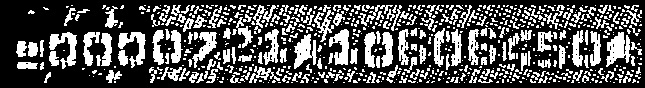
Next images show the results for each layer with and without backpropagation.

Original image

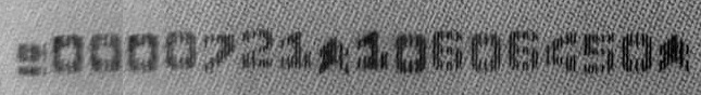
Transformed image
1st-pass using default parameters
Layer #0
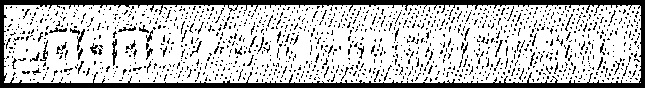
Layer #1
Layer #2
Layer #3
2nd-pass using refined parameters from backpropagation
Layer #0
Layer #1
Layer #2
Layer #3